GUDHI Python modules documentation

Data structures for cell complexes
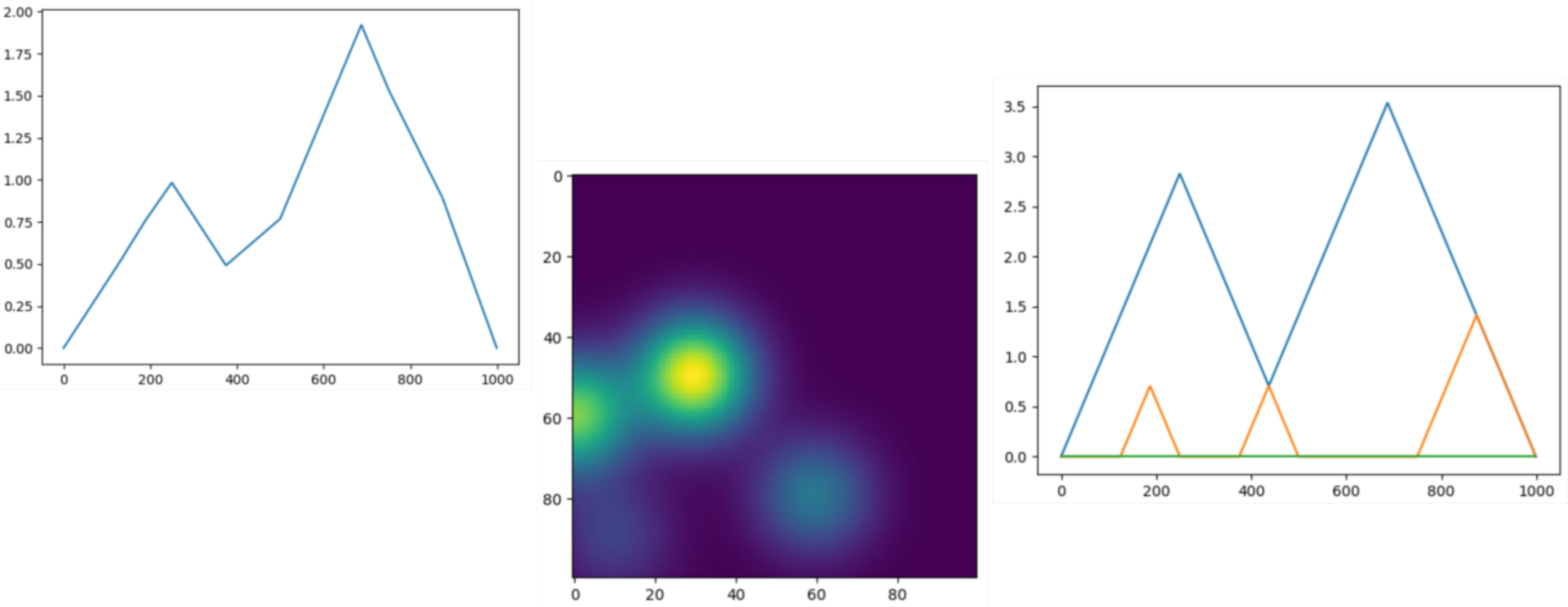
Cubical complexes

|
The cubical complex is an example of a structured complex useful in computational mathematics (specially rigorous numerics) and image analysis. |
|
Filtrations and reconstructions
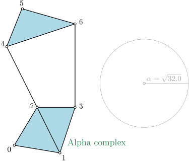
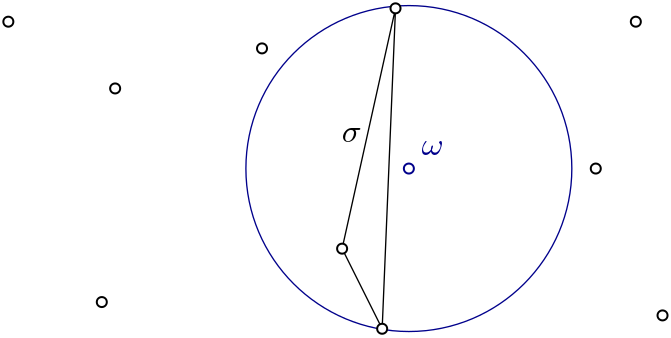
Alpha complex
|
Alpha complex is a simplicial complex constructed from the finite cells of a Delaunay Triangulation. The filtration value of each simplex is computed as the square of the circumradius of the simplex if the circumsphere is empty (the simplex is then said to be Gabriel), and as the minimum of the filtration values of the codimension 1 cofaces that make it not Gabriel otherwise. For performances reasons, it is advised to use CGAL \(\geq\) 5.0.0. |
|
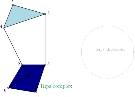
Rips complex
|
Rips complex is a simplicial complex constructed from a one skeleton graph. The filtration value of each edge is computed from a user-given distance function and is inserted until a user-given threshold value. This complex can be built from a point cloud and a distance function, or from a distance matrix. Weighted Rips complex constructs a simplicial complex from a distance matrix and weights on vertices. |
|
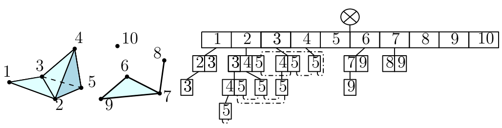
Witness complex
|
Witness complex \(Wit(W,L)\) is a simplicial complex defined on two sets of points in \(\mathbb{R}^D\). The data structure is described in [4]. |
|
Cover complexes
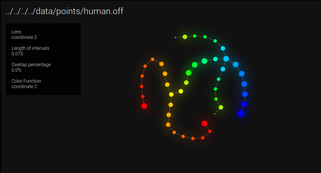
|
Nerves and Graph Induced Complexes are cover complexes, i.e. simplicial complexes that provably contain topological information about the input data. They can be computed with a cover of the data, that comes i.e. from the preimage of a family of intervals covering the image of a scalar-valued function defined on the data. |
|
Tangential complex
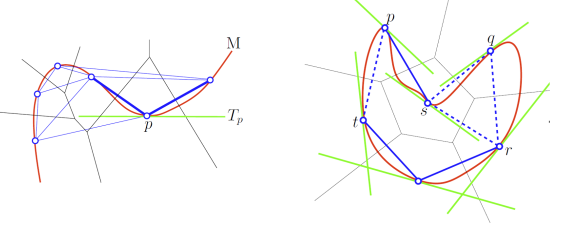
|
A Tangential Delaunay complex is a simplicial complex designed to reconstruct a \(k\)-dimensional manifold embedded in \(d\)- dimensional Euclidean space. The input is a point sample coming from an unknown manifold. The running time depends only linearly on the extrinsic dimension \(d\) and exponentially on the intrinsic dimension \(k\). |
|
Topological descriptors computation
Persistence cohomology
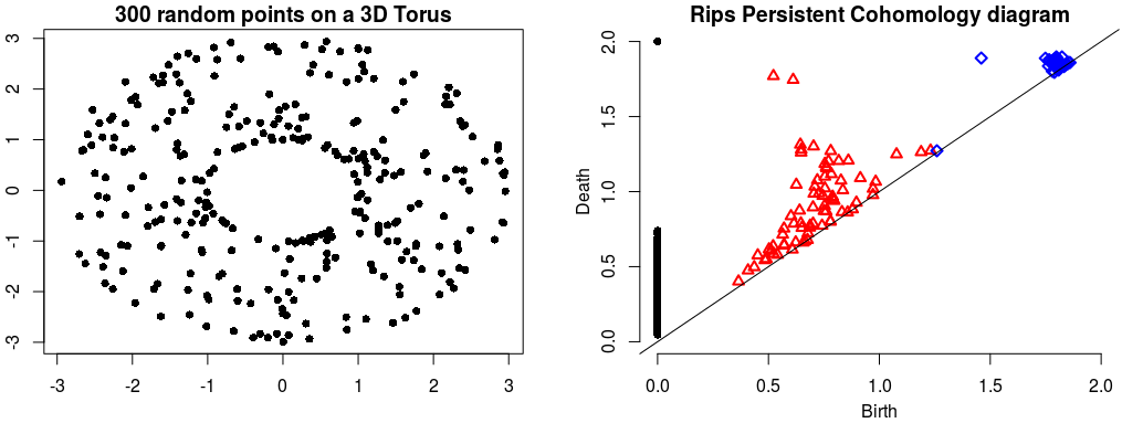
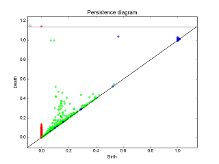
Rips Persistent Cohomology on a 3D Torus¶ |
The theory of homology consists in attaching to a topological space a sequence of (homology) groups, capturing global topological features like connected components, holes, cavities, etc. Persistent homology studies the evolution – birth, life and death – of these features when the topological space is changing. Consequently, the theory is essentially composed of three elements: topological spaces, their homology groups and an evolution scheme. Computation of persistent cohomology using the algorithm of [13] and [16] and the Compressed Annotation Matrix implementation of [2]. |
|
Please refer to each data structure that contains persistence feature for reference: |
||
Topological descriptors tools
Bottleneck distance
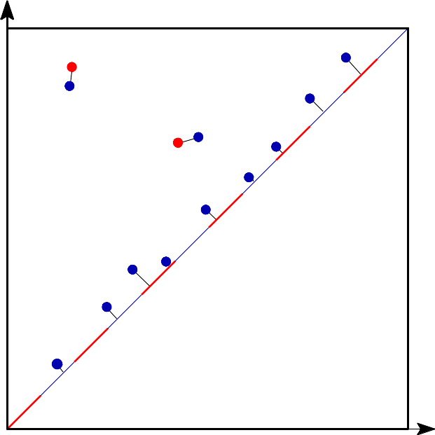
Bottleneck distance is the length of the longest edge¶ |
Bottleneck distance measures the similarity between two persistence diagrams. It’s the shortest distance b for which there exists a perfect matching between the points of the two diagrams (+ all the diagonal points) such that any couple of matched points are at distance at most b, where the distance between points is the sup norm in \(\mathbb{R}^2\). |
|
Wasserstein distance
|
|
The q-Wasserstein distance measures the similarity between two persistence diagrams using the sum of all edges lengths (instead of the maximum). It allows to define sophisticated objects such as barycenters of a family of persistence diagrams. |
|
Persistence representations
|
Vectorizations, distances and kernels that work on persistence diagrams, compatible with scikit-learn. |
|
Persistence graphical tools
|
These graphical tools comes on top of persistence results and allows the user to display easily persistence barcode, diagram or density. Note that these functions return the matplotlib axis, allowing for further modifications (title, aspect, etc.) |
|
Point cloud utilities
\((x_1, x_2, \ldots, x_d)\)
\((y_1, y_2, \ldots, y_d)\)
|
Utilities to process point clouds: read from file, subsample, find neighbors, embed time series in higher dimension, etc. |
|