Rips complex user manual#
Definition#
|
The Vietoris-Rips complex is a simplicial complex built as the clique-complex of a proximity graph. We also provide sparse approximations, to speed-up the computation of persistent homology, and weighted versions, which are more robust to outliers. |
|

|
||
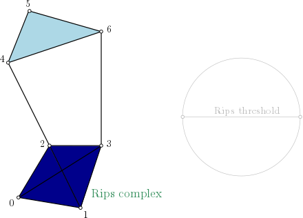
The Rips complex is a simplicial complex that generalizes proximity (\(\varepsilon\)-ball) graphs to higher dimensions. The vertices correspond to the input points, and a simplex is present if and only if its diameter is smaller than some parameter α. Considering all parameters α defines a filtered simplicial complex, where the filtration value of a simplex is its diameter. The filtration can be restricted to values α smaller than some threshold, to reduce its size. Beware that some people define the Rips complex using a bound of 2α instead of α, particularly when comparing it to an ambient Čech complex. They end up with the same combinatorial object, but filtration values which are half of ours.
The input discrete metric space can be provided as a point cloud plus a distance function, or as a distance matrix.
When creating a simplicial complex from the graph, RipsComplex first builds the graph and inserts it into the data structure. It then expands the simplicial complex (adds the simplices corresponding to cliques) when required. The expansion can be stopped at dimension max_dimension, by default 1.
A vertex name corresponds to the index of the point in the given range (aka. the point cloud).
Rips-complex one skeleton graph representation#
On this example, as edges (4,5), (4,6) and (5,6) are in the complex, simplex (4,5,6) is added with the filtration value set with \(max(filtration(4,5), filtration(4,6), filtration(5,6))\). And so on for simplex (0,1,2,3).
A Rips complex can easily become huge, even if we limit the length of the edges
and the dimension of the simplices. One easy trick, before building a Rips
complex on a point cloud, is to call sparsify_point_set() which removes points
that are too close to each other. This does not change its persistence diagram
by more than the length used to define “too close”.
A more general technique is to use a sparse approximation of the Rips
introduced by Don Sheehy [27]. We are using the version
described in [6] (except that we multiply all filtration
values by 2, to match the usual Rips complex). [10] proves
a \(\frac{1}{1-\varepsilon}\)-interleaving, although in practice the
error is usually smaller. A more intuitive presentation of the idea is
available in [10], and in a video
[11]. Passing an extra argument sparse=0.3 at the
construction of a RipsComplex object asks it to build a sparse Rips with
parameter \(\varepsilon=0.3\), while the default sparse=None builds the
regular Rips complex.
Another option which is especially useful if you want to compute persistent homology in “high” dimension (2 or more,
sometimes even 1), is to build the Rips complex only up to dimension 1 (a graph), then use
collapse_edges() to reduce the size of this graph, and finally call
expansion() to get a simplicial complex of a suitable dimension to compute its homology. This
trick gives the same persistence diagram as one would get with a plain use of RipsComplex, with a complex that is
often significantly smaller and thus faster to process.
Point cloud#
Example from a point cloud#
This example builds the neighborhood graph from the given points, up to max_edge_length. Then it creates a SimplexTree with it.
Finally, it is asked to display information about the simplicial complex.
import gudhi
rips_complex = gudhi.RipsComplex(points=[[1, 1], [7, 0], [4, 6], [9, 6], [0, 14], [2, 19], [9, 17]],
                                 max_edge_length=12.0)

simplex_tree = rips_complex.create_simplex_tree(max_dimension=1)
result_str = 'Rips complex is of dimension ' + repr(simplex_tree.dimension()) + ' - ' + \
    repr(simplex_tree.num_simplices()) + ' simplices - ' + \
    repr(simplex_tree.num_vertices()) + ' vertices.'
print(result_str)
fmt = '%s -> %.2f'
for filtered_value in simplex_tree.get_filtration():
    print(fmt % tuple(filtered_value))
When launching (Rips maximal distance between 2 points is 12.0, is expanded until dimension 1 - one skeleton graph in other words), the output is:
Rips complex is of dimension 1 - 18 simplices - 7 vertices.
[0] -> 0.00
[1] -> 0.00
[2] -> 0.00
[3] -> 0.00
[4] -> 0.00
[5] -> 0.00
[6] -> 0.00
[2, 3] -> 5.00
[4, 5] -> 5.39
[0, 2] -> 5.83
[0, 1] -> 6.08
[1, 3] -> 6.32
[1, 2] -> 6.71
[5, 6] -> 7.28
[2, 4] -> 8.94
[0, 3] -> 9.43
[4, 6] -> 9.49
[3, 6] -> 11.00
Notice that if we use
rips_complex = gudhi.RipsComplex(points=[[1, 1], [7, 0], [4, 6], [9, 6], [0, 14], [2, 19], [9, 17]],
                                 max_edge_length=12.0, sparse=2)
asking for a very sparse version (theory only gives some guarantee on the meaning of the output if sparse<1), 2 to 5 edges disappear, depending on the random vertex used to start the sparsification.
Example step by step#
While RipsComplex is convenient, for instance to build a simplicial complex in one line
import gudhi
points = [[1, 1], [7, 0], [4, 6], [9, 6], [0, 14], [2, 19], [9, 17]]
cplx = gudhi.RipsComplex(points=points, max_edge_length=12.0).create_simplex_tree(max_dimension=2)
you can achieve the same result without this class for more flexibility
import gudhi
from scipy.spatial.distance import cdist
points = [[1, 1], [7, 0], [4, 6], [9, 6], [0, 14], [2, 19], [9, 17]]
distance_matrix = cdist(points, points)
cplx = gudhi.SimplexTree.create_from_array(distance_matrix, max_filtration=12.0)
cplx.expansion(2)
or
import gudhi
from scipy.spatial import cKDTree
points = [[1, 1], [7, 0], [4, 6], [9, 6], [0, 14], [2, 19], [9, 17]]
tree = cKDTree(points)
edges = tree.sparse_distance_matrix(tree, max_distance=12.0, output_type="coo_matrix")
cplx = gudhi.SimplexTree()
cplx.insert_edges_from_coo_matrix(edges)
cplx.expansion(2)
This way, you can easily add a call to reduce_graph() before the insertion,
use a different metric to compute the matrix, or other variations.
Distance matrix#
Example from a distance matrix#
This example builds the one skeleton graph from the given distance matrix, and max_edge_length value. Then it creates a SimplexTree with it.
Finally, it is asked to display information about the simplicial complex.
import gudhi
rips_complex = gudhi.RipsComplex(distance_matrix=[[],
                                                  [6.0827625303],
                                                  [5.8309518948, 6.7082039325],
                                                  [9.4339811321, 6.3245553203, 5],
                                                  [13.0384048104, 15.6524758425, 8.94427191, 12.0415945788],
                                                  [18.0277563773, 19.6468827044, 13.152946438, 14.7648230602, 5.3851648071],
                                                  [17.88854382, 17.1172427686, 12.0830459736, 11, 9.4868329805, 7.2801098893]],
                                 max_edge_length=12.0)

simplex_tree = rips_complex.create_simplex_tree(max_dimension=1)
result_str = 'Rips complex is of dimension ' + repr(simplex_tree.dimension()) + ' - ' + \
    repr(simplex_tree.num_simplices()) + ' simplices - ' + \
    repr(simplex_tree.num_vertices()) + ' vertices.'
print(result_str)
fmt = '%s -> %.2f'
for filtered_value in simplex_tree.get_filtration():
    print(fmt % tuple(filtered_value))
When launching (Rips maximal distance between 2 points is 12.0, is expanded until dimension 1 - one skeleton graph in other words), the output is:
Rips complex is of dimension 1 - 18 simplices - 7 vertices.
[0] -> 0.00
[1] -> 0.00
[2] -> 0.00
[3] -> 0.00
[4] -> 0.00
[5] -> 0.00
[6] -> 0.00
[2, 3] -> 5.00
[4, 5] -> 5.39
[0, 2] -> 5.83
[0, 1] -> 6.08
[1, 3] -> 6.32
[1, 2] -> 6.71
[5, 6] -> 7.28
[2, 4] -> 8.94
[0, 3] -> 9.43
[4, 6] -> 9.49
[3, 6] -> 11.00
In case this lower triangular matrix is stored in a CSV file, like data/distance_matrix/full_square_distance_matrix.csv in the Gudhi distribution, you can read it with read_lower_triangular_matrix_from_csv_file().
Correlation matrix#
Example from a correlation matrix#
Analogously to the case of distance matrix, Rips complexes can be also constructed based on correlation matrix. Given a correlation matrix M, comportment-wise 1-M is a distance matrix. This example builds the one skeleton graph from the given corelation matrix and threshold value. Then it creates a SimplexTree with it.
Finally, it is asked to display information about the simplicial complex.
import gudhi
import numpy as np

# User defined correlation matrix is:
# |1     0.06    0.23    0.01    0.89|
# |0.06  1       0.74    0.01    0.61|
# |0.23  0.74    1       0.72    0.03|
# |0.01  0.01    0.72    1       0.7 |
# |0.89  0.61    0.03    0.7     1   |
correlation_matrix=np.array([[1., 0.06, 0.23, 0.01, 0.89],
                            [0.06, 1., 0.74, 0.01, 0.61],
                            [0.23, 0.74, 1., 0.72, 0.03],
                            [0.01, 0.01, 0.72, 1., 0.7],
                            [0.89, 0.61, 0.03, 0.7, 1.]], float)

distance_matrix = 1 - correlation_matrix
rips_complex = gudhi.RipsComplex(distance_matrix=distance_matrix, max_edge_length=1.0)

simplex_tree = rips_complex.create_simplex_tree(max_dimension=1)
result_str = 'Rips complex is of dimension ' + repr(simplex_tree.dimension()) + ' - ' + \
    repr(simplex_tree.num_simplices()) + ' simplices - ' + \
    repr(simplex_tree.num_vertices()) + ' vertices.'
print(result_str)
fmt = '%s -> %.2f'
for filtered_value in simplex_tree.get_filtration():
    print(fmt % tuple(filtered_value))
When launching (Rips maximal distance between 2 points is 12.0, is expanded until dimension 1 - one skeleton graph in other words), the output is:
Rips complex is of dimension 1 - 15 simplices - 5 vertices.
[0] -> 0.00
[1] -> 0.00
[2] -> 0.00
[3] -> 0.00
[4] -> 0.00
[0, 4] -> 0.11
[1, 2] -> 0.26
[2, 3] -> 0.28
[3, 4] -> 0.30
[1, 4] -> 0.39
[0, 2] -> 0.77
[0, 1] -> 0.94
[2, 4] -> 0.97
[0, 3] -> 0.99
[1, 3] -> 0.99
Note
If you compute the persistence diagram and convert distances back to correlation values, points in the persistence diagram will be under the diagonal, and bottleneck distance and persistence graphical tool will not work properly, this is a known issue.
Weighted Rips Complex#
WeightedRipsComplex builds a simplicial complex from a distance matrix and weights on vertices.
Example from a distance matrix and weights#
The following example computes the weighted Rips filtration associated with a distance matrix and weights on vertices.
from gudhi.weighted_rips_complex import WeightedRipsComplex
dist = [[], [1]]
weights = [1, 100]
w_rips = WeightedRipsComplex(distance_matrix=dist, weights=weights)
st = w_rips.create_simplex_tree(max_dimension=2)
print(list(st.get_filtration()))
The output is:
[([0], 2.0), ([1], 200.0), ([0, 1], 200.0)]
Example from a point cloud combined with DistanceToMeasure#
Combining with DistanceToMeasure, one can compute the DTM-filtration of a point set, as in this notebook. Remark that DTMRipsComplex class provides exactly this function.
import numpy as np
from scipy.spatial.distance import cdist
from gudhi.point_cloud.dtm import DistanceToMeasure
from gudhi.weighted_rips_complex import WeightedRipsComplex
pts = np.array([[2.0, 2.0], [0.0, 1.0], [3.0, 4.0]])
dist = cdist(pts,pts)
dtm = DistanceToMeasure(2, q=2, metric="precomputed")
r = dtm.fit_transform(dist)
w_rips = WeightedRipsComplex(distance_matrix=dist, weights=r)
st = w_rips.create_simplex_tree(max_dimension=2)
print(st.persistence())
The output is:
[(0, (3.1622776601683795, inf)), (0, (3.1622776601683795, 5.39834563766817)), (0, (3.1622776601683795, 5.39834563766817))]
DTM Rips Complex#
DTMRipsComplex builds a simplicial complex from a point set or a full distance matrix (in the form of ndarray), as described in the above example.
This class constructs a weighted Rips complex giving larger weights to outliers, which reduces their impact on the persistence diagram. See this notebook for some experiments.
import numpy as np
from gudhi.dtm_rips_complex import DTMRipsComplex
pts = np.array([[2.0, 2.0], [0.0, 1.0], [3.0, 4.0]])
dtm_rips = DTMRipsComplex(points=pts, k=2)
st = dtm_rips.create_simplex_tree(max_dimension=2)
print(st.persistence())
The output is:
[(0, (3.1622776601683795, inf)), (0, (3.1622776601683795, 5.39834563766817)), (0, (3.1622776601683795, 5.39834563766817))]