Cover complexes user manual
Definition
|
Nerves and Graph Induced Complexes are cover complexes, i.e. simplicial complexes that provably contain topological information about the input data. They can be computed with a cover of the data, that comes i.e. from the preimage of a family of intervals covering the image of a scalar-valued function defined on the data. |
|
Visualizations of the simplicial complexes can be done with either neato (from graphviz), geomview, KeplerMapper. Input point clouds are assumed to be OFF files (cf. OFF file format).
Covers
Nerves and Graph Induced Complexes require a cover C of the input point cloud P, that is a set of subsets of P whose union is P itself. Very often, this cover is obtained from the preimage of a family of intervals covering the image of some scalar-valued function f defined on P. This family is parameterized by its resolution, which can be either the number or the length of the intervals, and its gain, which is the overlap percentage between consecutive intervals (ordered by their first values).
Nerves
Nerve definition
Assume you are given a cover C of your point cloud P. Then, the Nerve of this cover is the simplicial complex that has one k-simplex per k-fold intersection of cover elements. See also Wikipedia.
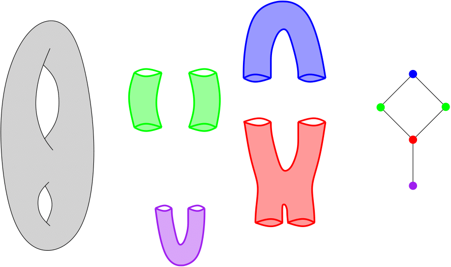
Nerve of a double torus
Example
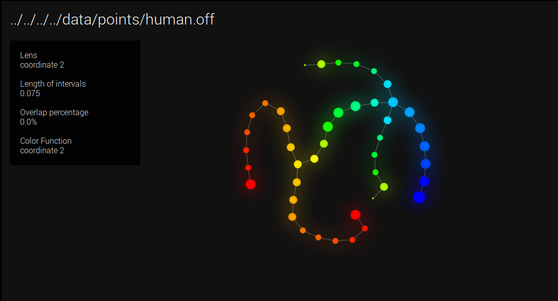
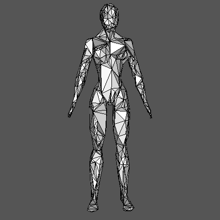
This example builds the Nerve of a point cloud sampled on a 3D human shape (human.off). The cover C comes from the preimages of intervals (10 intervals with gain 0.3) covering the height function (coordinate 2), which are then refined into their connected components using the triangulation of the .OFF file.
import gudhi
nerve_complex = gudhi.CoverComplex()
nerve_complex.set_verbose(True)

if (nerve_complex.read_point_cloud(gudhi.__root_source_dir__ + \
'/data/points/human.off')):
    nerve_complex.set_type('Nerve')
    nerve_complex.set_color_from_coordinate(2)
    nerve_complex.set_function_from_coordinate(2)
    nerve_complex.set_graph_from_OFF()
    nerve_complex.set_resolution_with_interval_number(10)
    nerve_complex.set_gain(0.3)
    nerve_complex.set_cover_from_function()
    nerve_complex.find_simplices()
    nerve_complex.write_info()
    simplex_tree = nerve_complex.create_simplex_tree()
    nerve_complex.compute_PD()
    result_str = 'Nerve is of dimension ' + repr(simplex_tree.dimension()) + ' - ' + \
        repr(simplex_tree.num_simplices()) + ' simplices - ' + \
        repr(simplex_tree.num_vertices()) + ' vertices.'
    print(result_str)
    for filtered_value in simplex_tree.get_filtration():
        print(filtered_value[0])
the program output is:
Min function value = -0.979672 and Max function value = 0.816414
Interval 0 = [-0.979672, -0.761576]
Interval 1 = [-0.838551, -0.581967]
Interval 2 = [-0.658942, -0.402359]
Interval 3 = [-0.479334, -0.22275]
Interval 4 = [-0.299725, -0.0431414]
Interval 5 = [-0.120117, 0.136467]
Interval 6 = [0.059492, 0.316076]
Interval 7 = [0.239101, 0.495684]
Interval 8 = [0.418709, 0.675293]
Interval 9 = [0.598318, 0.816414]
Computing preimages...
Computing connected components...
5 interval(s) in dimension 0:
  [-0.909111, 0.0081753]
  [-0.171433, 0.367393]
  [-0.171433, 0.367393]
  [-0.909111, 0.745853]
0 interval(s) in dimension 1:
Nerve is of dimension 1 - 41 simplices - 21 vertices.
[0]
[1]
[4]
[1, 4]
[2]
[0, 2]
[8]
[2, 8]
[5]
[4, 5]
[9]
[8, 9]
[13]
[5, 13]
[14]
[9, 14]
[19]
[13, 19]
[25]
[32]
[20]
[20, 32]
[33]
[25, 33]
[26]
[14, 26]
[19, 26]
[42]
[26, 42]
[34]
[33, 34]
[27]
[20, 27]
[35]
[27, 35]
[34, 35]
[35, 42]
[44]
[35, 44]
[54]
[44, 54]
The program also writes a file ../../data/points/human.off_sc.txt. The first three lines in this file are the location of the input point cloud and the function used to compute the cover. The fourth line contains the number of vertices nv and edges ne of the Nerve. The next nv lines represent the vertices. Each line contains the vertex ID, the number of data points it contains, and their average color function value. Finally, the next ne lines represent the edges, characterized by the ID of their vertices.
Using KeplerMapper, one can obtain the following visualization:
Visualization with KeplerMapper
Graph Induced Complexes (GIC)
GIC definition
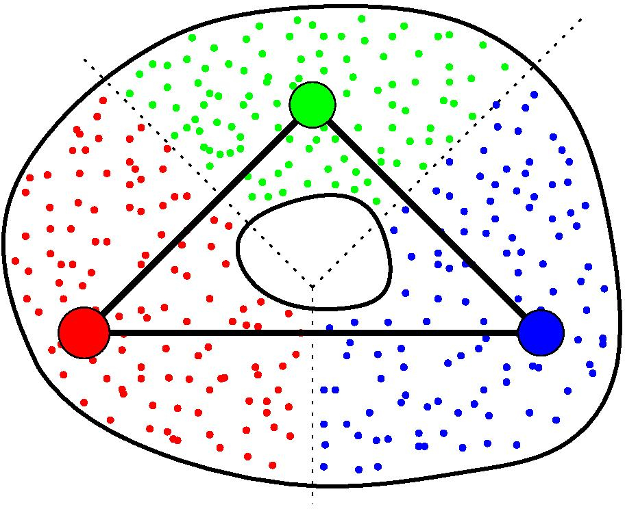
Again, assume you are given a cover C of your point cloud P. Moreover, assume you are also given a graph G built on top of P. Then, for any clique in G whose nodes all belong to different elements of C, the GIC includes a corresponding simplex, whose dimension is the number of nodes in the clique minus one. See [15] for more details.
GIC of a point cloud
Example with cover from Voronoï
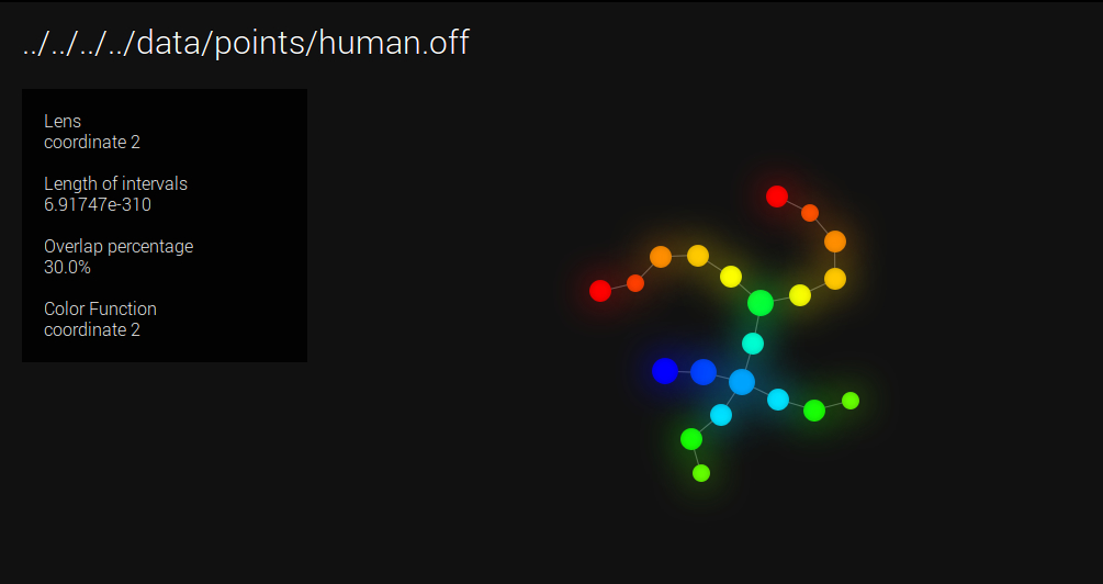
This example builds the GIC of a point cloud sampled on a 3D human shape (human.off). We randomly subsampled 100 points in the point cloud, which act as seeds of a geodesic Voronoï diagram. Each cell of the diagram is then an element of C. The graph G (used to compute both the geodesics for Voronoï and the GIC) comes from the triangulation of the human shape. Note that the resulting simplicial complex is in dimension 3 in this example.
import gudhi
nerve_complex = gudhi.CoverComplex()

if (nerve_complex.read_point_cloud(gudhi.__root_source_dir__ + \
'/data/points/human.off')):
    nerve_complex.set_type('GIC')
    nerve_complex.set_color_from_coordinate()
    nerve_complex.set_graph_from_OFF()
    nerve_complex.set_cover_from_Voronoi(700)
    nerve_complex.find_simplices()
    nerve_complex.plot_off()
the program outputs SC.off. Using e.g.
geomview ../../data/points/human.off_sc.off
one can obtain the following visualization:
Visualization with Geomview
Functional GIC
If one restricts to the cliques in G whose nodes all belong to preimages of consecutive intervals (assuming the cover of the height function is minimal, i.e. no more than two intervals can intersect at a time), the GIC is of dimension one, i.e. a graph. We call this graph the functional GIC. See [8] for more details.
Example
Functional GIC comes with automatic selection of the Rips threshold, the resolution and the gain of the function cover. See [7] for more details. In this example, we compute the functional GIC of a Klein bottle embedded in R^5, where the graph G comes from a Rips complex with automatic threshold, and the cover C comes from the preimages of intervals covering the first coordinate, with automatic resolution and gain. Note that automatic threshold, resolution and gain can be computed as well for the Nerve.
import gudhi
nerve_complex = gudhi.CoverComplex()

if (nerve_complex.read_point_cloud(gudhi.__root_source_dir__ + \
'/data/points/KleinBottle5D.off')):
    nerve_complex.set_type('GIC')
    nerve_complex.set_color_from_coordinate(0)
    nerve_complex.set_function_from_coordinate(0)
    nerve_complex.set_graph_from_automatic_rips()
    nerve_complex.set_automatic_resolution()
    nerve_complex.set_gain()
    nerve_complex.set_cover_from_function()
    nerve_complex.find_simplices()
    nerve_complex.plot_dot()
the program outputs SC.dot. Using e.g.
neato ../../data/points/KleinBottle5D.off_sc.dot -Tpdf -o ../../data/points/KleinBottle5D.off_sc.pdf
one can obtain the following visualization:
Visualization with neato
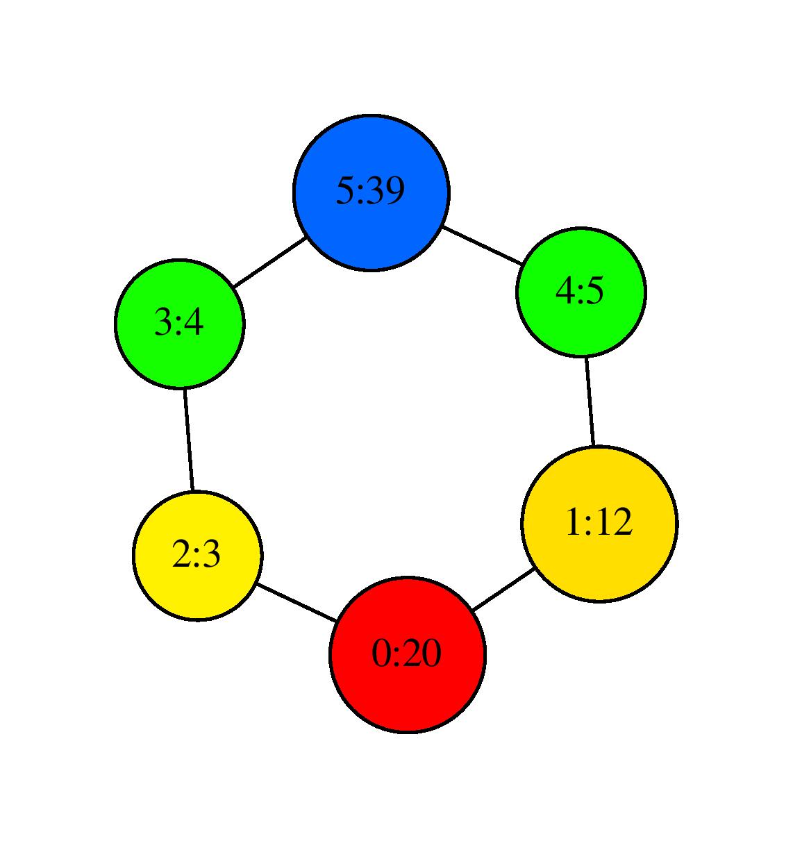
where nodes are colored by the filter function values and, for each node, the first number is its ID and the second is the number of data points that its contain.
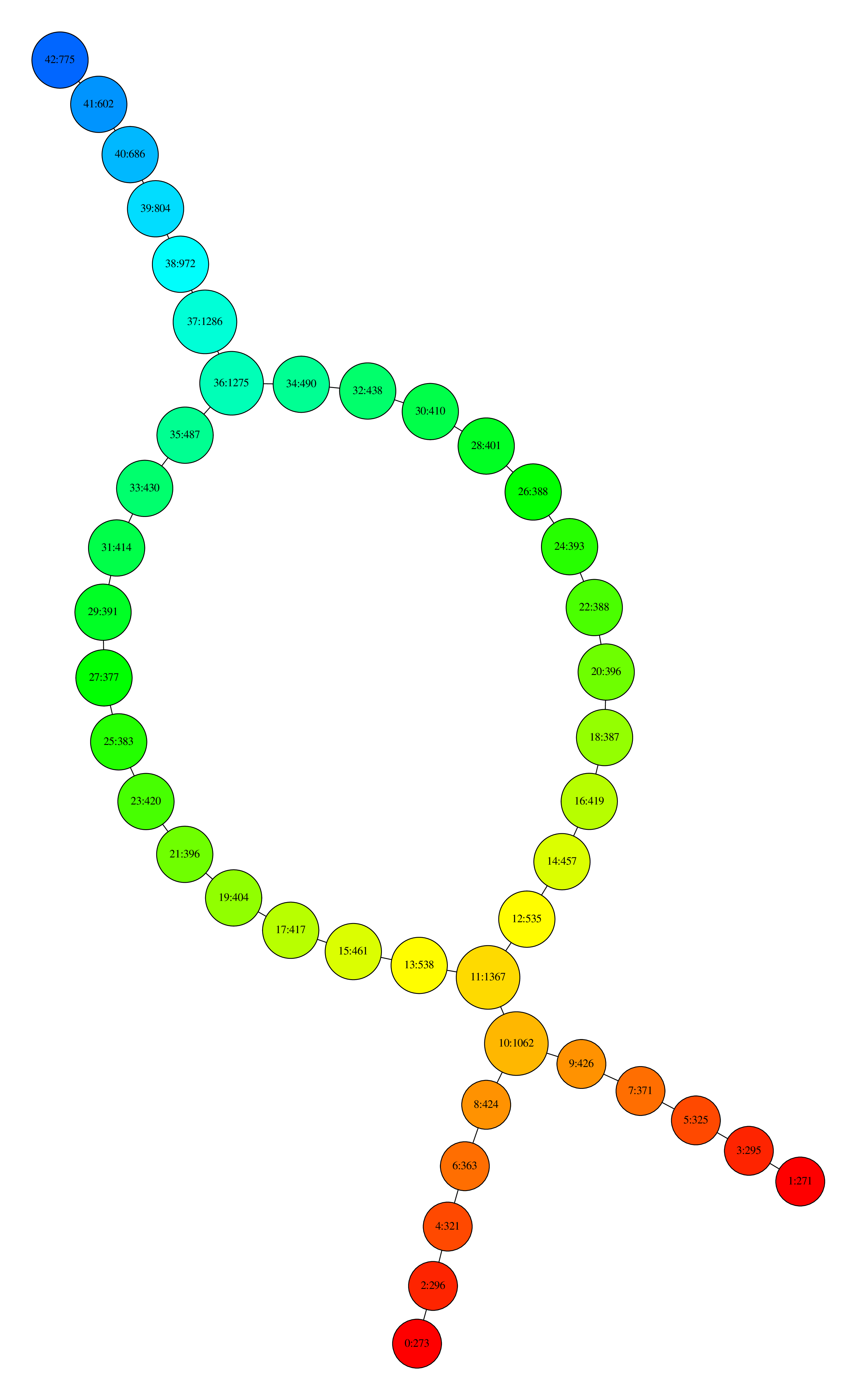
We also provide an example on a set of 72 pictures taken around the same object (lucky_cat.off). The function is now the first eigenfunction given by PCA, whose values are written in a file (lucky_cat_PCA1). Threshold, resolution and gain are automatically selected as before.
import gudhi
nerve_complex = gudhi.CoverComplex()

if (nerve_complex.read_point_cloud(gudhi.__root_source_dir__ + \
'/data/points/COIL_database/lucky_cat.off')):
    nerve_complex.set_type('GIC')
    pca_file = gudhi.__root_source_dir__ + \
    '/data/points/COIL_database/lucky_cat_PCA1'
    nerve_complex.set_color_from_file(pca_file)
    nerve_complex.set_function_from_file(pca_file)
    nerve_complex.set_graph_from_automatic_rips()
    nerve_complex.set_automatic_resolution()
    nerve_complex.set_gain()
    nerve_complex.set_cover_from_function()
    nerve_complex.find_simplices()
    nerve_complex.plot_dot()
the program outputs again SC.dot which gives the following visualization after using neato:
Visualization with neato